Rare Earth Magnet Basics / Rare Earth Magnet Basics
Click the thumbnails for the large figure.
An aggregation of mini-magnets with north and south poles (magnetic dipoles) is called a magnetic body. Material in the world is made of atoms, molecules, and other particles that are affected by magnetic action and these are magnetic dipoles. Thus, it can be said that ultimately all material is some type of magnetic material or other. Among these, those materials that have particularly strong magnetic dipoles and that furthermore have special magnetic properties that give them practical value are called magnetic materials. Special magnetic properties means the values for the magnetic properties of saturation magnetization, permeability, and coercive force. This will be explained in detail later.
Material that can become magnetic material has distinctive ways of lining up the magnetic dipoles.
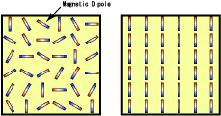
Figure (a) Ordinary Material(Left)
Figure (b) Ferromagnetic Body(Right)

Table (a) Types of Magnetic Bodies
Figure (a) is a schematic diagram of the arrangement of magnetic dipoles in ordinary material. These magnetic dipoles are oriented randomly in all in directions, so this is not a strongly magnetic material.
On the other hand,in Figure (b), the magnetic dipoles are all lined up in one direction. Since a material that has such a structure can demonstrate strong magnetism, this magnetic characteristic is called ferromagnetic. There are two types of material that demonstrate ferromagnetism: ferromagnetic bodies and ferrimagnetic bodies.
When magnetic materials actually used are classified from the perspective of function, there are generally two types. One is called soft magnetic materials and the other is called hard magnetic materials. Here, soft and hard are named according to how the magnetic dipoles within each type of material react to external magnetic fields.
Figure (c)is a schematic diagram of these materials. When an external magnetic field H is applied to a magnetic body, if the magnetic dipoles in the material easily orient in the direction of the applied magnetic field and easily follow the direction of the external magnetic field, this material is called a soft magnetic material. On the other hand, a material that does not line up with the direction of the external magnetic field but rather keeps the magnetic dipoles aligned in a specific direction even when the magnetic field direction changes is called a hard magnetic material.

Figure (c) Types of Magnetic Materials
For magnetic materials, the value that expresses the degree of ease of orienting the magnetic dipoles to the direction of the external magnetic field, the degree to which the dipoles follow the field, is called the magnetic permeability. The easier the orientation of the magnetic dipoles changes, the higher magnetic permeability. On the other hand, materials for which the orientation of the magnetic dipoles is difficult to change are considered to have low magnetic permeability.
Materials with magnetic dipoles with large magnetic moments and low small magnetic permeability and that are stable relative to external magnetic fields are used as permanent magnets. With permanent magnets, even if you apply a large external magnetic field, the orientation of the magnetic dipoles does not change and the state of orienting in a specific direction (direction of easy magnetization) is maintained. The above coercive force is a value expressing the degree of difficulty of changing this arrangement. The larger the coercive force, the greater the stability of the magnet and the less it is changed even by a large external magnetic field.
Table (b) shows the main types of permanent magnetic materials currently used in industry.
The main components of ferrite magnets are oxides of iron (Fe), barium (Ba), and strontium (Sr). Because these materials are cheap, they hold costs down and since the main components are oxides, they provide such features as high specific electric resistance and superior corrosion resistance.
On the other hand, alloy magnets include alnico magnets and rare earth magnets. In particular, rare earth magnets were developed from the second half of the 1960s and have extraordinarily high magnetic characteristics compared to other permanent magnetic materials. Rare earth magnets include samarium cobalt (SmCo) magnets and neodymium iron boron (NdFeB) magnets. More details on these magnets can be found on the home page.
When permanent magnetic materials are used, in addition to the magnetic materials being used alone, sometimes they are powdered, mixed with plastic or rubber, and molded. Such magnets are called bonded magnets. Bonded magnets can be freely processed into any shape and can be formed into a single piece with other parts, but since the proportion of magnetic material within the total volume is less, their magnetic force is reduced to the same degree.
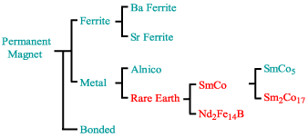
Table (b) Types of Permanent Magnets
4. -1 Magnetization Curves and Hysteresis Loops
Next, we will consider methods for quantitatively evaluating magnetic characteristics. The magnetic flux density B, magnetic field H, and magnetization J (I) within magnets and various other magnetidies have the following relationships.
B =μ0H + J ( B = H + 4πI )*
B : Magnetic flux density [ T ] ( [ G ] )
H : Magnetic field [ A / m ] ( [ Oe ] )
J ( I ) : Magnetization [ T ] ( [ G ] )
μ0 : Magnetic permeability of vacuum 4π×10-7 [ H / m ]
( * This page shows physical quantities and equations expressed in SI units. For reference, the CGS Gauss system values are given in parentheses. )
This equation shows that the magnetic flux density B within a magnetic body is expressed by the sum H of the magnitude of the magnetic field and the magnetization J (I) of the magnetic body. Since the magnitude of the magnetic field H is normally known, in order to find the magnitude of the magnetic flux density B, the magnetization J (I) of the magnetic body is found. The magnitude of the magnetization J (I) of the magnetic body varies with the magnitude of the magnetic field. A drawing showing this relationship is called a J-H loop (4πI-H loop).
Figure (d) shows the J-H loop (4πI-H loop) for a permanent magnet. The value of the external magnetic field H applied to the material is plotted on the horizontal axis and the value of the magnetization J of the material induced by the external magnetic field is plotted on the vertical axis. The relationship between this magnetization J and external magnetic field H varies with the sequence followed by the material, so this is called a hysteresis loop. When a magnetic field is applied to a permanent magnet in the state in which the magnetization J is 0 (neutral state), as the magnetic field increases, the magnetization also increases steadily. When a large enough magnetic field has been created, the magnet reaches saturation. The curve 0-a-b-c for this is called the initial magnetization curve and creating a permanent magnet from the neutral state in this way is called magnetizing. The magnitude of the magnetization at Point c where the magnet is completely magnetized and can not be magnetized further is called the saturation magnetization Js (4πIs) .
From the state in which the magnetization has reached saturation, if the external magnetic field is now reduced, the magnetization does not pass along the original curve, but rather decreases gradually as in c-d. The magnitude of the magnetization at Point d when the magnetic field is 0 is called the remanent magnetization Jr (4πIr) . If the magnetic field is further reduced, even if the magnetic field is increased in the direction opposite to that for the magnetization direction, the magnetization does not immediately become 0. This is a feature of a hard magnetic material. When the magnetic field is decreased, the magnetization traces a curve like d-e-f and the magnetic field at Point f is 0. The magnitude of the magnetic field when the magnetization is 0 is called the coercive force HcJ . The curve d-e-f is called the demagnetization curve.
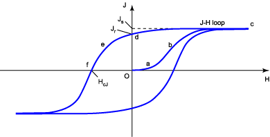
Figure (d) Permanent Magnet J-H Loop (4πI-H loop)
When evaluating the magnetic properties of a permanent magnet itself, the demagnetization curve (J-H curve (4πI-H curve)) in an adequately magnetized state is used. On the other hand, in the actual usage state for the material, in addition to the magnetization J of the material, the external magnetic field H is also taken into account and sometimes it is more appropriate to evaluate with the B-H curve which shows the relationship between the magnetic flux density B and the external magnetic field H.
Figure (e) shows a permanent magnet J-H loop (4πI-H loop) and B-H loop. As mentioned earlier, the flux density B is the constant multiple of the magnetic field H added to the magnetization J (4πI), so compared to the J-H loop (4πI-H loop), the B-H loop has a higher right shoulder.
In the demagnetization curve, left on the normal magnetic field H axis is positive. The value of the magnetic flux density when the magnetic field in the figure on the left is 0 is called the remanent flux density Br. This value is the same as the remanent magnetization Jr (4πIr) . The magnitude of the magnetic field for which the magnetic flux density becomes 0 is called the coercive force, the same as for the magnitude of the magnetic field when the magnetization becomes 0 mentioned above. The coercive force when the magnetic flux density becomes 0 is written as HcB to distinguish it from the coercive force HcJ for when the magnetization becomes 0.

Figure (e) J-H loop (4πI-H loop) and B-H loop
4. -2 Demagnetization Field and Permeance Coefficient
As in Figure (f), within a magnet with a finite shape, the magnetization of the material itself generates a magnetic field in the opposite direction from the direction of the magnetization, a demagnetization field Hd. When an attempt is made to extract magnetic flux from a magnetic material, this demagnetization field always exists as long as the size of the material is finite. The magnitude of this demagnetization field Hd is proportional to the magnitude of the magnetization and is expressed as:
Hd = - NJ/μ0 ( Hd = - N4πI )
N : Demagnetizing factor
The demagnetizing factor N is determined by the shape of the magnetic body.
Normally, analysis of a magnetic field uses the B-H curve, so instead of this demagnetizing factor N, the permeance coefficient defined as
p = - Bd / μ0Hd ( p = - Bd / Hd )
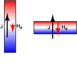
Figure (f) Shape of Magnet and Demagnetization Field

Figure (g) Demagnetization Field and Permeance Line
is used. Here, as in Bd Figure (g), Bd is the value of the magnetic flux density when the demagnetization field Hd is the magnetic field on the B-H curve. This permeance coefficient is determined by the shape of the magnetic body, just like the demagnetizing factor N. The relationship between the permeance coefficient and the demagnetizing factor N is as below.
p = ( 1 - N ) / N
Also, the straight line OP passing between the origin and the Hd and Bd) points on the B-H curve is called the permeance line. The slope of this line is the permeance coefficient p.
4. -3 Maximum Energy Product of a Magnet
The magnitude of energy that can be taken out from a magnet is proportional to the product of the magnetic flux density B and the magnetic field H on the B-H curve in Figure (h). The maximum value of this product of the magnetic flux density B and the magnetic field H is called the maximum energy product (BH)max and its units are kJ / m3 (MGOe) . To be a powerful magnet, in other words a magnet with a large maximum energy product, the remanent flux density Br and coercive force HcB on the B-H curve must be large. To express this in terms of the J-H curve (4πI-H curve), the larger the remanent magnetization Jr and the coercive force HcJ and the more nearly square the J-H curve (4πI-H curve), the more superior the magnet.
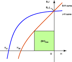
Figure (h) B-H Curve, J-H Curve (4πI-H curve), and (BH)max
When the temperature of a magnetized magnet is changed from room temperature T1 to a high temperature T2, the fluctuation of the magnetic moment due to thermal energy changes the demagnetization curve as in Figure (i). Accompanying this, the remanent flux density Br and coercive force HcJ decrease. This decrease of the magnetic flux density B is called flux loss.
As Table (c) shows, there are two types of flux loss: reversible flux loss, in which the magnetic flux density returns to its original magnitude when the magnet's temperature is returned to room temperature T1, and irreversible flux loss, in which the magnetic flux density does not return to its original magnitude even when the magnet's temperature is returned to room temperature T1.

Figure (i) Temperature Change for J-H
Curve (4πI-H Curve) and B-H Curve
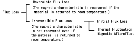
Table (c) Types of Flux Loss
5. -1 Reversible Flux Loss
For reversible flux loss, the degree of change of the remanent flux density Br and of the coercive force HcJ with temperature depends on the type of rare earth magnet. The temperature coefficients are in the characteristics table.
5. -2 Irreversible Flux Loss
Irreversible flux loss, in which the magnetic flux density does not completely return to its original magnitude even when the temperature of the magnet is returned to room temperature T1, has two types.
5. -2-1 Initial Flux Loss
Now, the demagnetization curve in Figure (j) for a certain magnet at room temperature is (1) and the demagnetization curve for the same magnet at higher temperature is (2). First, if the usage permeance coefficient for that magnet is p1, then its working point is shifted temporarily from Point a to Point b by higher temperature, but is returned to Point a by cooling. (Reversible flux loss) However, if the usage permeance coefficient is p2, the working point, which had been at Point a', is shifted by higher temperature to Point b', which is below the knee of the curve. In this case, the working point that has shifted does not return to its original Point a' even when the magnet is cooled, but rather only recovers to Point c. The resulting flux loss a'-c is called the initial flux loss.
The degree of this initial flux loss, the same as for reversible flux loss, is determined by the type of rare earth magnet, the usage temperature, and the usage permeance coefficient.

Figure (j) B-H Curve Temperature Change
and Permeance Line
5. -2-2 Thermal Fluctuation Magnetic Aftereffect
The magnetization of a magnetized magnet gradually decreases over time due to thermal fluctuation of the magnetic moment. This is called thermal fluctuation magnetic aftereffect. The magnitude of this phenomenon varies, but it occurs in all types of magnets given a long enough time. In other words, what we call "permanent magnets" are not "permanently magnets". The smaller the permeance coefficient of the magnetic circuit the magnet is used in and the higher the temperature at which that magnetic circuit is used, the greater the flux loss.